Detecting the Shine-Dalgarno Sequence
A Computational Genomics assignment
Aim
The goal of this post is to report the results of a Hidden Markov Model (HMM) from known ribosomal binding sites in E. coli and then applying the model to (parts of) the genome to establish potential binding partners in the sequence.
1. What does the transition probabilities SN->S1 and SN->SN represent in terms of our assumptions about RBS in the genome? How would changes to these values affect the performance of the model?
That we assume RBS will occur twice every 1000 nucleotides in the sequence. An increase in the transition probability between SN -> S1 would increase the chance of more RBSs being detected (regardless of whether they were true or false), in other words, it would increase the number of true predictions but it will lower precision.
2. For the emission probabilities in states S1-S14, what are the highest observed frequencies? Can you discover the Shine-Delgarno (SD) sequence in these probabilities? Why are these values not 100% for the SD components?
The emissions (rounded to the second digit) are computed as below:
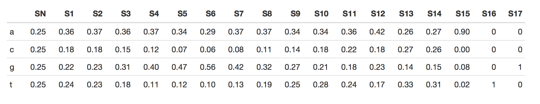
The highest observed frequencies for S1-S14 are:
- g : 56% in State 6
- g : 47% in State 5
- a : 42% in State 12
- g : 42% in State 7
- g : 40% in State 4
The Shine-Delgarno sequence in Escherichia coli is a base of AGGAGG, and based on observation, one could say that the SD sequence is mostly around S4 - S9.
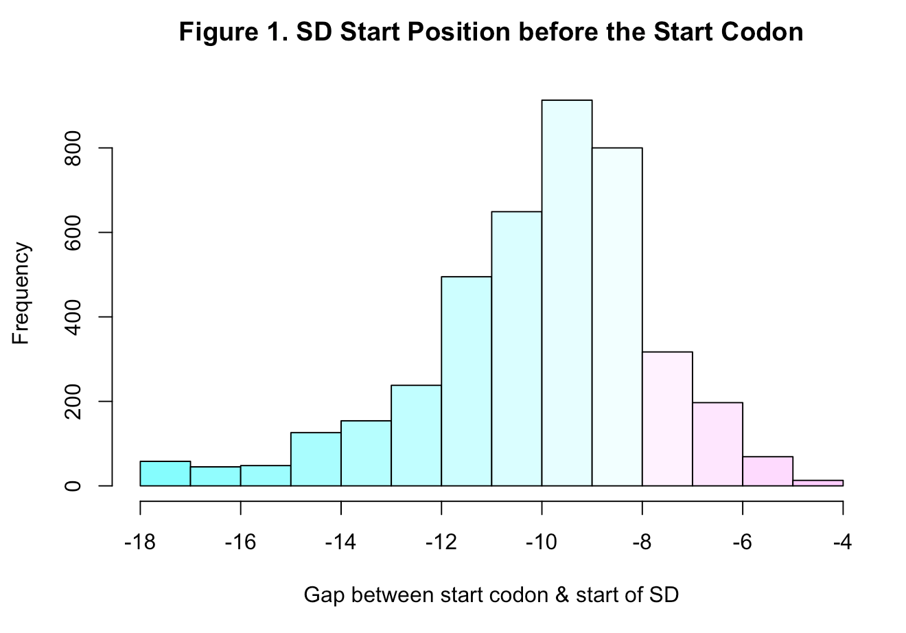
While the SD sequence is mostly 6 consecutive nucleotides, they aren’t really exactly located 7 or 8 bp before the start codon. As seen in the histogram below (data taken from sd_table.txt ), most SDs appear around 8 bp before the transcript site yet are diversly located anywhere between 18 to 4 bp prior. So that entails that the state emissions probabilities are just approximations, they don’t account for the beginninng of the SD and that’s why they’re not a 100% for all.
3. How could the model be changed to model the SD sequence a bit more closely in the data?
To begin with, the inclusion of all of the 33 states should improve the model, since a portion of start positions of SD are in that region (before the 14 selected states). Moreover, emission should be factored to calculate the entropy/strength of presence of the SD based on the distances between them and the start codon (ATG). That way, the strong presence of SD in the most anticipated regions/states will be “magnified” through the emission rates.
Dynamic Programming
Displaying Model as a BED File
Using a python script that converts the Viterbi solution to a BED file, displaying through IGV (with the loading of the E. coli K-12 genome). We inspect the sites of the predicted RBSs in IGV.
What’s true and what’s false?
It would be difficult to discern with confidence, however, here are a few analysed results:
As the sequence AGGAGG is 83% present starting on the second state, one could say it’s a true binding site.
This could be highly perceived as a false BDS, the reason being that the emission rates reflected are not accurate, hence the site suited the model because the states had nucleotides that relfected the not-so-accurate emission rates (i.e. State 13 had a high rate for T (33%), states 9-12 also hold high percentages for A, hence, the site (falsely) looked probable to the model).
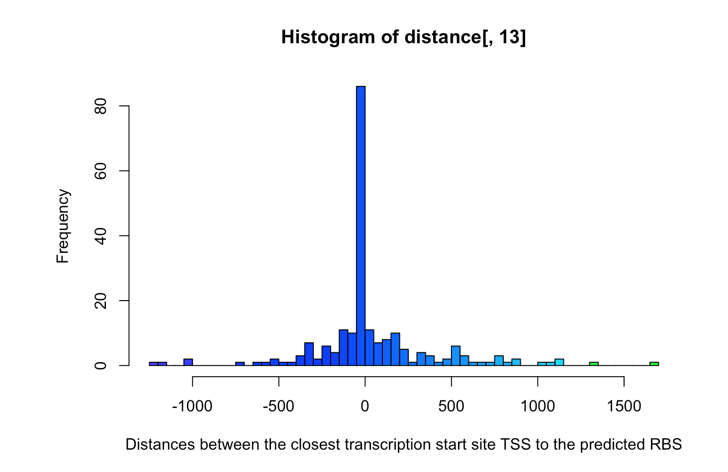
2. Use Bedtools to establish the closest transcription start site TSS to each predicted RBS (e.g. closestBed –D b –a rbs.bed –b ecoli_tss.bed). Summarise the resulting distance distribution (a histogram or density plot might do well here). The distance is reported in the last column of the output. Argue how you would rate the overall results coming from the HMM:
The overall results aren’t satisfactory (low precision and low recall) and the model need improvement.
False positive rate
```{r echo=FALSE} num <- which(distance[,13] != 0)
frate <- length(num)/dim(distance)[1] ```
The false positive rate is the number of times an SD has been predicted incorrectly. It can be calculated as follows:
(number of times the distance is not 0) / (number of SD predictions) = r length(num) / 270 = r frate
False positives
The mapping of the emission rates to the states as mentioned does not take into consideration the varying start positions of the SD sequence. So the emission rates are detecting variant sequences that resemble the Shine Dalgarno sequence partially, or even remotely if the other states that don’t encapsulate the SD nucleotides affect the result.
Reducing false RBS predictions
By improving the model in such a way that would account the detection for the actual SD position within the binding site. Assuming the actual emissions of the SD have been adjusted within the state emission rates (as illustrated in Question 2 yet without rounding, since some true values are lost that way), the state transition probability matrix can then be adjusted in such a way that would allow for transitions between the normal state and all the states, with high transition probability for states that hold a high probability of the SD start positions (i.e. based on figure 1, S6 (9 bp before the start codon S15) is the most likely state where the SD begins (if we take all 33 States, that would be equivalent to S23)).